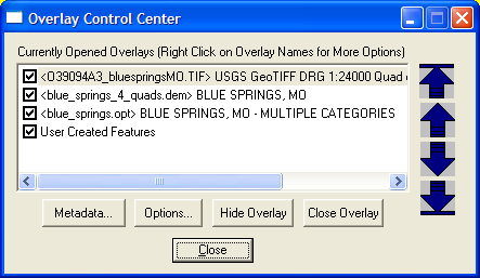
This is a list of the all currently opened overlays. You can select an overlay by clicking on its name. Multiple overlays can be selected using the shift and control keys while clicking on overlays in the list. If the overlay is currently hidden, it is indicated to the left of the overlay description. Double-clicking on a layer automatically brings up its Options dialog. If you hold down the 'M' key while double-clicking the Metadata dialog for the layer will be displayed instead.

You can right click on the list of currently opened overlays to display a list of options available to perform on the selected overlays. Examples of available options include the following:

Selecting the Create Elevation Grid from 3D Vector Data option on the popup menu that appears when right-clicking on vector layers in the Overlay Control Center displays the Elevation Grid Creation Options dialog, pictured below. Using this dialog, you can configure how you want the elevation grid to be created using the selected vector data as well as what portion of the selected overlays to use when creating the elevation grid. You can also use the Gridding tab to specify that your data should be gridded in sections. This makes it possible to grid data sets that are too large to grid all at once.

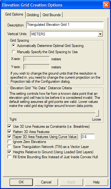
The following options are also available when generating the grid:

• Use 3D Line Features as Constraints (i.e. Breaklines) - If this option is checked, any line and area features that have elevation values associated with them will be treated as constraints/breaklines. This will ensure that elevation values along the line/area boundary will be consistent with the elevation that should be along the line.
• Flatten 3D Area Features - If you have any area/polygon features with elevation in the selected layers that you are gridding, they will be treated as flattened areas rather than just additional 3D data points/constraints. This allows you to create flattened areas like lakes and also nice terrain surfaces from things like building models. If only 3D area features are present, any grid locations outside of the areas will be marked as invalid, otherwise the grid locations within areas will just be flattened to the area heights and the remainder of the grid will be generated as usual.
• Taper 3D Area Features Using Curve Value - If you have any area/polygon features with elevation in the selected layers that you are gridding and you also checked the option to flatten 3D area features, the taper option allows you to specify that rather than making the areas absolutely flat, the edges should be tapered with the area elevation existing near the centroid of the area and the elevation applied for the area dwindling to zero as you reach the area edge. The curve value specifies the exponent to apply to the percent distance a sample location is between the area centroid and the area edge to adjust the height applied at that location. Values less than 1 will make the edge steepness progressively greater (i.e. flatter at the middle, then steep edges), while values larger than one cause the steepness to be near the area centroid and flatter towards the edges, while a value of 1 provides for a linear taper. For example if you want to simulate a sand bunker for a golf course, a value of around 0.5 provides a decent simulation of a bunker.
• Ignore Zero Elevations - If checked, this option will cause any features with an elevation value of zero to be ignored. This is useful if you have a data set where features with no known elevation are marked with an elevation of zero.
• Save Triangulated Network (TIN) as a Vector Layer - If checked, this option will cause a separate vector layer with area features for each 3D triangle created as part of the triangulation and gridding process. This is known as the TIN surface.
• Heights Relative to Ground - If you check this option, all elevation values from the selected vector layers will be treated as relative to the height of any loaded underlying terrain surface (like a DEM). This is very handy for doing things like creating building models where you just know the building height above ground and not above sea level.
• Fill Entire Bounding Box Instead of Just Inside Convex Hull - If you check this option, the generated elevation grid will contain valid values filling the entire bounding box specified for the gridding operation. Otherwise, the valid values will only fill out to the convex hull polygon of the data being gridded.
• Export Grids Directly to Global Mapper Grid Files - If checked, this option will cause the generated elevation grid file(s) to be directly exported to Global Mapper Grid (GMG) files. This is useful when you are triangulating and gridding a very large collection of data and also using the Gridding tab to split the operation into smaller pieces. By directly exporting the results to GMG files you can create elevation grids that normally would not all fit into memory.

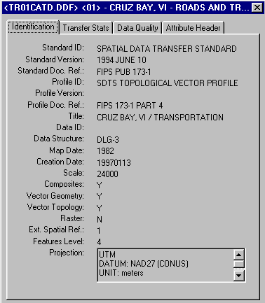
Pressing the Metadata... button displays metadata for the selected overlay. The actual metadata dialog displayed depends on the type of the selected overlay. The metadata dialog for a SDTS DLG is shown below.

Pressing the Options... button displays a dialog containing the available display options for the selected overlay(s). Options can be set on multiple raster or elevation overlays at the same time. The available display options depend on the type of the selected overlays. The following display options are used:

Selecting the Options... button while a vector (i.e. SHP, DXF, E00, etc) overlay is selected displays the Vector Options dialog (pictured below).

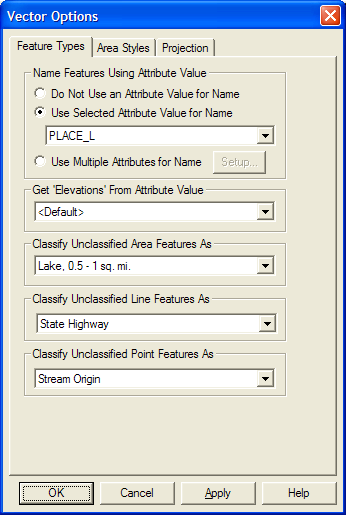
The Feature Types tab provides the ability to specify which attribute field(s) (if any) to display as the name of features loaded from the vector file. You can also select which attribute field (if any) to use for the "elevation" value for the layer. By default, several attribute field names (like "ELEVATION", "ELEV", "ALTITUDE", "Z", etc.) are checked when an elevation value for the feature is needed. This option allows you to override this behavior and manually select the attribute to use. Finally, there are also options available to select the classification to apply to unclassified area, line, and/or point features in the layer.

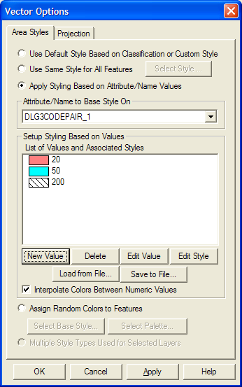
The Area Styles and Line Styles tabs provide the ability to customize how area and line features found in the selected layer(s) are displayed. The following style settings are available:

The Projection tab is used to reinterpret the raw vector data to a new projection. This is useful if the wrong projection was selected for the dataset when it was loaded, or if the data set itself indicated some incorrect data. This option is rarely used. You can however also use the Elevation Units control to specify what elevation units that values in the vector data that do not explicitly specify their units should use. This is useful to indicate if the values associated with 3D vector features or with the ELEVATION attribute for features are in feet or meters.

Selecting the Options... button while only raster overlays are selected displays the Raster Options dialog. The Raster Options dialog consists of several tabs, each allowing you to control various aspects of how the selected raster layers are displayed.

The Display tab (pictured below) contains controls allowing you to control the color intensity (brightness/darkness), color transparency, blending, anti-aliasing, and texture mapping of the selected layers.

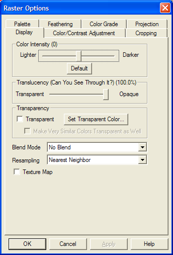
The Color Intensity setting controls whether displayed pixels are lightened or darkened before being displayed. It may be useful to lighten or darken raster overlays in order to see overlaying vector data clearly.

The Translucency setting controls to what degree you can see through the overlay to overlays underneath the overlay. The default setting of Opaque means that you cannot see through the overlay at all. Settings closer to Transparent make the overlay increasingly more see-through, allowing you to blend overlapping data.

The Blend Mode setting controls how an overlay is blended with underlying overlays, in addition to the Translucency setting. These settings allow Photoshop-style filters to be applied to overlays, resulting in often stunning results. What you get from a particular set of overlays from a particular blend mode setting can often be hard to predict, so rather than try to understand what is technically happening for each blend mode it's best to just experiment with different ones until you find one that you like. The Hard Light setting seems to work well with satellite imagery overlaid on DEMs, but the others can be quite useful as well. For example, the Apply Color setting is useful for applying color to a grayscale overlay, such as using a low-resolution color LANDSAT image to colorize a high-resolution grayscale satellite image. The SPOT Natural Color blend mode combines the color channels in the topmost layer using the common algorithm for generating natural color imagery from images from the SPOT HRV multi-spectral sensor [Red = B2; Green = ( 3 * B1 + B3 ) / 4; Blue = ( 3 * B1 - B3 ) / 4]. The Pseudo Natural Color blend mode combines the color channels within a single image using a common algorithm for generating natural color imagery from CIR imagery.

The Transparent option allows a particular color (or colors) to be displayed transparently, making it possible to see through a layer to the layers underneath. For example, when viewing a DRG on top of a DOQ, making the white in the DRG transparent makes it possible to see much of the DOQ underneath. Pressing the Set Transparent Color... button allows the user to select the color (or multiple colors for palette-based files) to treat as transparent in the selected overlay(s) as well as save the palette for palette-based files to a color palette (.pal) file. If you also check the Make Very Similar Colors Transparent as Well option, any colors that are a very similar color to the selected transparent color will also be displayed transparently. This is useful for getting rid of colors in lossy formats like JPG and ECW where the colors are not exact.

The Resampling option allows you to control how the color value for each displayed/export location is determined based on the values in the file. The following resampling methods are supported:

• Nearest Neighbor - simply uses the value of the sample/pixel that a sample location is in. When resampling or reprojected an image this can result in a stair-step effect, but will maintain exactly the original color values of the source image.
• Bilinear Interpolation - determines the value of a new pixel based on a weighted average of the 4 pixels in the nearest 2 x 2 neighborhood of the pixel in the original image. The averaging has an anti-aliasing effect and therefore produces relatively smooth edges with hardly any jaggies.
• Bicubic Interpolation - a more sophisticated method that produces smoother edges than bilinear interpolation. Here, a new pixel is a bicubic function using 16 pixels in the nearest 4 x 4 neighborhood of the pixel in the original image. This is the method most commonly used by image editing software, printer drivers and many digital cameras for resampling images.
• Box Average (3x3, 4x4, and 5x5) - the box average methods simply find the average values of the nearest 9 (for 3x3), 16 (for 4x4), or 25 (for 5x5) pixels and use that as the value of the sample location. These methods are very good for resampling data at lower resolutions. The lower the resolution of your export is as compared to the original, the larger "box" size you should use.

The Texture Map option allows a 2D raster overlay to be draped over loaded 3D elevation overlays. Selecting the check box causes the overlay to use any available data from underlying elevation layers to determine how to color the DRG or DOQ. The result is a shaded relief map.

The Color/Contrast Adjustment tab (pictured below) allows you to control the color balance and contrast of the selected overlay(s).

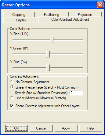
The Color Balance sliders allow you modify the relative amounts of red, green, and blue in the image, thus allowing precise control over the color balance in the image.

The Contrast Adjustment options are used to adjust the contrast of imagery. The Linear (Percentage Stretch) contrast adjustment method applies a standard deviation contrast adjust to each color channel in the image. You can specify how many standard deviations from the mean that the range is stretch to for rendering, although you'll generally want to stick with the default of 2. This is particularly useful for improving the display of dark or satellite imagery, such as IKONOS images, and is required for the display of imagery with more than 8 bits per color channe. The Linear (Min/Max Stretch) method finds the minimum and maximum values in each color channel and stretches that range to a range of 0 to 255. For most imagery with 8 bits or less per color channel this will have no effect, but can produce a good result for high-color imagery.

The Share Contrast Adjustment with Other Layers checkbox allows you to specify that the calculated contrast adjustment used should be based on all loaded raster layers that have contrast adjustment enabled rather than just the color histogram for this single layer. This is enabled by default and provides consistent results when adjusting the contrast for multiple mosaiced images.

The Cropping tab (pictured below) allows you to crop the selected overlay(s) to a particular boundary, including support for automatically removing the collars from USGS DRG topographic maps.

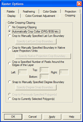
The Automatically Crop Collar (DRG/BSB/etc.) option is used to automatically remove the collar from loaded raster data if the collar is in a recognized format. Most frequently it is used to removes the white border around a DRG, the small black collar around a 3.75 minute DOQQ, or the map collar around a BSB marine chart. This allows you to seamlessly view a collection of adjacent BSB, DRG, or DOQQ files.

The Crop to Manually Specified Lat/Lon Boundary option allows you to specify a lat/lon boundary (in the native datum of the selected overlay) to crop the overlay to. When selected, this option will display the Customize Collar Bounds dialog (pictured below) to allow specifying the bounds to crop to.

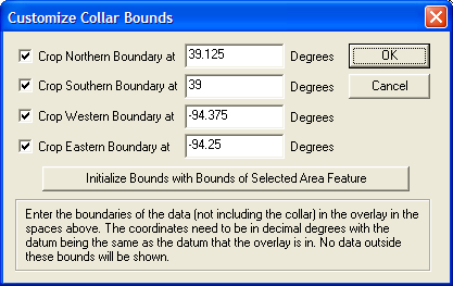
The Crop to Manually Specified Boundary in Native Layer Projection/Units option allows you to specify a crop boundary in the native units of the selected overlay. When selected, this option will display the Customize Collar Bounds dialog (pictured above) to allow specifying the bounds to crop to.

The Crop a Specified Number of Pixels Around the Edges of the Layer option allows you to specify a number of pixels to crop of each edge of the selected overlay(s).

The Snap to Manually Specified Degree Boundary option allows you to specify that the collar for the selected overlay will be on some degree boundary, like an even degree, of 0.5 degrees, etc. This way you can setup cropping for a collection of maps that are all similarly aligned.

The Crop to Previously Selected Polygon(s) option specifies that you want to crop to the crop polygon(s) (area) previously applied to the selected layer(s) using the Crop to Currently Selected Polygon option.

The Crop to Currently Selected Polygon(s) option specifies that you want to crop the selected layer(s) to any area feature(s) currently selected with either the Feature Info or Digitizer Tools.

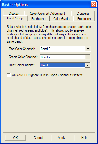
The Band Setup tab (pictured below) is available for some types of imagery with 3 or more bands of data. This tab allows you to control which bands of data are used for the red, green, and blue color bands. This is a very useful tool when trying to extract different types of information out of multi-spectral imagery.

There is also an option for advanced users to allow disabling of the alpha (translucency) channel for an image. This is useful if you have an image with bad alpha values (like all set to completely transparent) and you just want to see the colors without applying the alpha values.

The Palette tab (pictured below) is available for raster image files that use a fixed color palette for display. This tab allows you to see what colors are in the palette as well as edit the color and/or description of each color in the palette. This allows you to easily replace one color with another. You can also save the palette to a new file or load an entirely new palette to use for the layer from an existing .PAL or .CLR file.

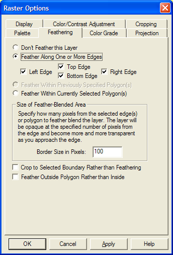
The Feathering tab (pictured below) allows you specify that you would like to feather-blend the selected overlay(s) with the underlying overlay(s) on the specified edges. This can be extremely powerful tool for blending imagery/maps from different sources and/or at different resolution to make the edge between the map sets invisible. You can choose to either feather-blend around the edges of selected files or along the boundary of one or more selected polygons. Feather blending can be used on both raster (imagery) layers as well as gridded elevation layers. In the case of elevation layers, the feather blending works by calculating modified elevation values based on elevation value in the blended layer and the topmost elevation layer underneath the blended layer in the draw order.

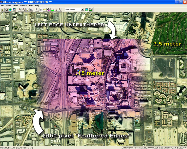
The screenshot below displays the results of feather-blending a very high resolution data set (0.15 meters per pixel) with a lower resolution (3.5 meters per pixel) dataset to remove the edge. Note that the higher resolution image has been purposely tinted violet to make the effect more obvious.

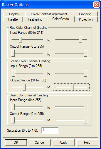
The Color Grade tab (pictured below) allows you to apply complex color correction to a loaded raster file. You can setup the input range for each color channel and what output range to map it to, as well as specify a saturation value.

Selecting the Options... button while only gridded elevation overlays are selected displays the Elevation Options dialog. The Elevation Options dialog consists of two tabs, one for controlling the display of the overlay(s) and the other for modifying the elevation values within the overlay(s).

The Display tab (pictured below) contains controls allowing you to control the color intensity (brightness/darkness), color transparency, blending, anti-aliasing, and color shading of the selected layers.

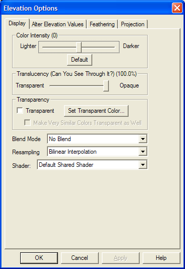
The Color Intensity setting controls whether displayed pixels are lightened or darkened before being displayed. It may be useful to lighten or darken raster overlays in order to see overlaying vector data clearly.

The Translucency setting controls to what degree you can see through the overlay to overlays underneat the overlay. The default setting of Opaque means that you cannot see through the overlay at all. Settings closer to Transparent make the overlay increasingly more see-through, allowing you to blend overlapping data.

The Blend Mode setting controls how an overlay is blended with underlying overlays, in addition to the Translucency setting. These settings allow Photoshop-style filters to be applied to overlays, resulting in often stunning results. What you get from a particular set of overlays from a particular blend mode setting can often be hard to predict, so rather than try to understand what is technically happening for each blend mode it's best to just experiment with different ones until you find one that you like. The Hard Light setting seems to work well with satellite imagery overlaid on DEMs, but the others can be quite useful as well.

The Transparent option allows a particular color to be displayed transparently, making it possible to see through a layer to the layers underneath. For example, when viewing a DRG on top of a DOQ, making the white in the DRG transparent makes it possible to see much of the DOQ underneath. Pressing the Set Transparent Color... button allows the user to select the color to treat as transparent in the selected overlay.

The Resampling option allows you to control how the elevation value for each displayed/export location is determined based on the values in the file. The following resampling methods are supported:

• Nearest Neighbor - simply uses the value of the sample that a location is in. When resampling or reprojected an image this can result in a stair-step effect, but will maintain exactly the original elevation values of the source file.
• Bilinear Interpolation - determines the value of a new sample based on a weighted average of the 4 samples in the nearest 2 x 2 neighborhood of the sample in the original image. The averaging has an anti-aliasing effect and therefore produces relatively smooth edges with hardly any jaggies.
• Bicubic Interpolation - a more sophisticated method that produces smoother edges than bilinear interpolation. Here, a new pixel is a bicubic function using 16 samples in the nearest 4 x 4 neighborhood of the sample in the original image.
• Box Average (3x3, 4x4, and 5x5) - the box average methods simply find the average values of the nearest 9 (for 3x3), 16 (for 4x4), or 25 (for 5x5) samples and use that as the value of the sample location. These methods are very good for resampling data at lower resolutions. The lower the resolution of your export is as compared to the original, the larger "box" size you should use.

The Shader option allows you to choose which elevation shader is to be used for coloring the cell values within this layer. By default, all gridded layers will share the elevation shader selected on the toolbar, but there may be certain situations where you want to color one layer differently than the others and exclude it from the loaded elevation range. One common example is a gridded layer that actually has non-elevation data.

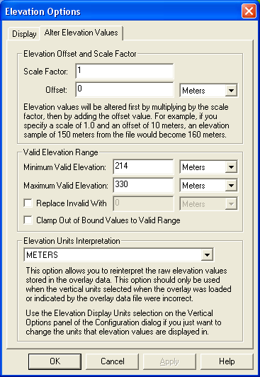
The Alter Elevation Values tab (pictured below) allows you to modify how elevation values from the selected layer(s) are interpreted, providing you a means to offset all of the elevations in the layer(s) by a given value and to restrict the range of elevation values that are treated as valid.

Toggles whether the currently selected overlays are visible. You can also use the checkboxes next to each layer to control the visible state of the overlays.

Closes all the currently selected overlays.